
🧮🖼 What should happen inside a missing region of an image?
Not “fill it with AI.”
Not “call a library.”
But mathematically — what should the pixel values be?
I wanted to answer that question from first principles.
The Physics Inspiration
In physics, the Laplace equation
$$ \nabla^2 u = 0 $$
describes steady-state heat flow, electrostatic potential, and incompressible fluid flow.
Its solutions are called harmonic functions — functions with zero curvature.
They smoothly interpolate boundary information without introducing oscillations.
That led to a modeling idea:
Treat the damaged image region like a steady-state physical system.
The Original Image
Here is the original image before any damage:

The Modeling Assumption
Suppose the image is a function ( u(x,y) ).
Inside the missing region:
$$ \nabla^2 u(x,y) = 0 $$
while known pixels act as Dirichlet boundary conditions.
This means the damaged region should extend surrounding pixel intensities with minimal curvature.
Not machine learning.
Just physics.
Artificial Damage (Diagonal Scratch)
To test the method, I introduced a thin diagonal scratch:

The masked region becomes the unknown domain where the Laplace equation must be solved.
From Physics to Computation
Using second-order central differences:
$$ \frac{\partial^2 u}{\partial x^2} \approx \frac{u_{i+1,j} - 2u_{i,j} + u_{i-1,j}}{h^2} $$
$$ \frac{\partial^2 u}{\partial y^2} \approx \frac{u_{i,j+1} - 2u_{i,j} + u_{i,j-1}}{h^2} $$
Substituting into the Laplace equation gives:
$$u_{i+1,j}+u_{i-1,j}+u_{i,j+1}+u_{i,j-1}-4u_{i,j}=0 $$
Rearranging:
$$ u_{i,j}= \frac{1}{4} \left( u_{i+1,j} + u_{i-1,j} + u_{i,j+1} + u_{i,j-1} \right) $$
Each missing pixel equals the average of its four neighbors.
A local rule that produces a global linear system:
$$ A \mathbf{u} = \mathbf{b} $$
Solving the System: Successive Over-Relaxation
To accelerate convergence, I used SOR:
$$ u_{i,j}^{(k+1)}=(1-\omega)u_{i,j}^{(k)} + \frac{\omega}{4} \left( u_{i+1,j} + u_{i-1,j} + u_{i,j+1} + u_{i,j-1} \right) $$
For ( 1 < \omega < 2 ), convergence accelerates significantly.
The relaxation parameter modifies the spectral radius of the iteration matrix, directly controlling convergence speed.
Before and After
Damaged Image
Inpainted (SOR)

Convergence Behavior
Here is the residual decay (log scale):
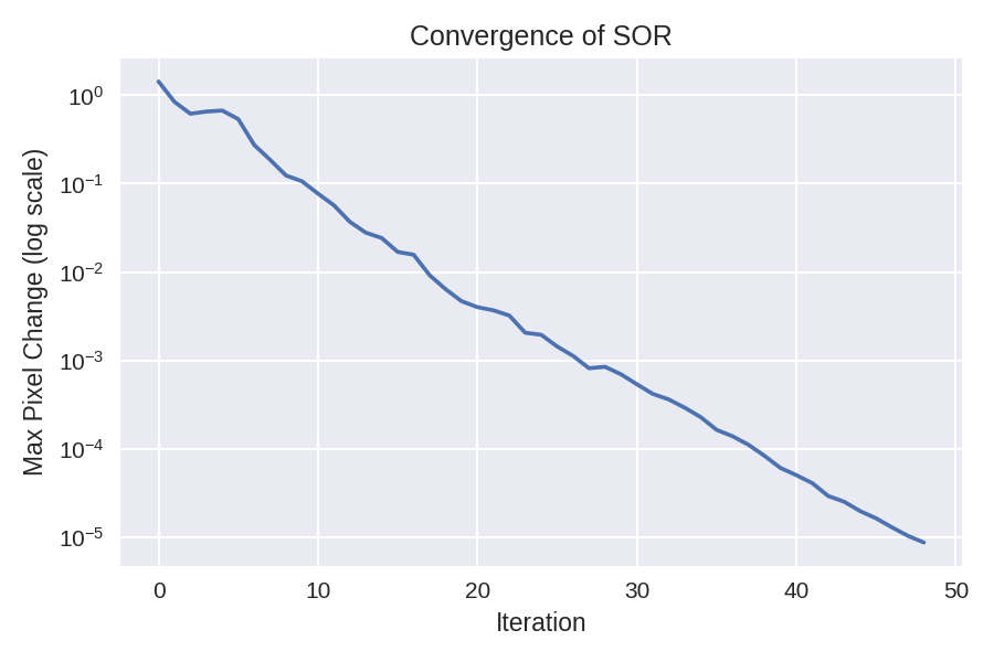
The exponential decay is characteristic of elliptic PDE discretizations with diagonal dominance.
Watching that curve flatten is deeply satisfying.
What This Method Can — and Cannot — Do
This approach produces:
- Smooth harmonic interpolation
- Stable convergence
- Physically consistent reconstruction
It does not:
- Recover fine textures
- Reconstruct sharp edges
- Invent new structure
It assumes smooth continuation.
Which is mathematically honest.
Why Build It from Scratch?
Libraries abstract away structure.
Building it manually reveals:
- Why diagonal dominance ensures convergence
- How sparsity makes large systems tractable
- How relaxation modifies convergence rate
- How numerical stability depends on matrix structure
The insight transfers directly to:
- Optimization algorithms
- Gradient-based methods
- Sparse linear solvers
- Scientific simulation
The math scales.
The API does not.
Closing Thought
Solving a PDE to repair an image is strangely satisfying.
You’re not guessing pixels.
You’re enforcing a physical law.
You’re letting structure propagate inward from the boundary.
And once you understand that structure,
you’re no longer just using tools —
you’re designing them.